Overview
The carbon loophole refers to the embodied greenhouse gas (GHG) emissions associated with the production of goods that are ultimately traded across countries. The term ‘embodied emissions’ refers to the total amount of emissions from all upstream processes required to deliver a certain product or service. These emissions are a growing issue for global efforts to decarbonize the world economy. Embodied emissions in trade are not accounted for in most current GHG accounting systems and climate policies. Under the UNFCCC, countries report their GHG emissions on the basis of territorial emissions (also called production-based emissions (PBA)). When goods and services are traded, the emissions associated with their production (or embodied emissions) are also traded, and these imported emissions are not counted towards the consumer country’s emissions reporting. As countries work toward net zero emissions, the relevance of emissions embodied in imported goods becomes more significant, precipitating increased awareness of the need to shift toward consumption-based accounting (CBA).
Emissions shifting manifests in several ways: new and existing emitters can relocate; a company can choose a different supplier to fulfill an order, or a decrease in domestic emissions can be more than compensated for by increased imports. The latter can occur when an economy shifts from an industrial base to an information or service economy, which increases physical imports to compensate for declining domestic production. The microeconomic decisions underlying emissions shifting are complex, and energy and pollution costs are only some of the variables that may influence businesses’ decision-making. These decisions will also vary by type of industry. Yet whatever the precise mechanics of emissions shifting, the problem is persistent and is growing in certain countries and regions. To prevent further burden-shifting, major economies must recognize that even strong regulation on domestic emissions in major economies may not be effective in reducing total global emissions due to their imported carbon, i.e. carbon loophole.
This could potentially hinder the global effort to reach the target of the Paris Climate Agreement: to limit global warming to “well below” 2 ℃. An alternative emissions attribution, consumption-based accounting, is proposed to correct this issue. This accounting perspective attributes emissions to the consumer of the final product, irrespective of where the production takes place.
While consumption-based emissions accounting seems to echo the equity and justice principle, its implementation has still been limited due to the complexity that occurs due to the involvement of bilateral and multilateral relations between countries. More local and national governments are trying to address the issue of carbon embodied in trade. For example, the Green Public Procurement (GPP) (also called Buy Clean) policies introduced in several countries and regions require that certain carbon-intensive infrastructure materials (e.g. steel, cement, concrete, etc.) purchased with government funds are produced below a given threshold of carbon intensity. Another example of such policies to address embodied carbon in trade is the carbon border adjustment. For example, the European Council officially accepted a framework for a carbon border adjustment mechanism (CBAM) seeking to reduce carbon leakage on imports, specifically targeting fertilizers, steel, iron, cement, aluminum, and electric energy production. These policies help level the playing field and provide a market for companies that have invested in low-carbon technologies for producing materials.
This tool provides essential data to the state of embodied carbon in international trade and global carbon emissions. The tool provides macro-analysis of embodied carbon in trade in certain countries/regions and for 24 key carbon-intensive products (see the list below).
We developed an Environmentally-Extended Multi-Regional Input-Output (EE MRIO) model to measure the part of the global CO2 emissions that are transferred through global trade. To be able to do this, we use the latest version of the EXIOBASE 3 database (3.8.2) (EXIOBASE 2022). We further refined the CO2 intensity of a few key subsectors for which we had good carbon intensity data (e.g. steel, aluminum, and cement). EXIOBASE is a global, detailed Multi-Regional Environmentally Extended Supply-Use Table (MR-SUT) and Input-Output Table (MR-IOT). It was developed by harmonizing and detailing supply-use tables for many countries, estimating emissions and resource extractions by industry. Subsequently, the country supply-use tables were linked via trade creating an MR-SUT and producing MR-IOTs from this. The MR-IOT can be used for the analysis of the environmental impacts associated with the final consumption of product groups. EXIOBASE 3 supplies a time series of EE MRIO tables of 44 countries and 5 rest-of-the-world regions, ranging from 1995 to 2022, with 163 economic sectors. We focus on analyzing CO2 emissions in this analysis. The EE MRIO model allows us to measure both the direct and indirect emissions embodied in domestic and foreign consumption (EXIOBASE 2022). For this study we only include CO2 emissions because of data limitation within EXIOBASE. It should be noted that EE MRIO model and analysis are based on monetary values for outputs and CO2 intensities (as opposed to physical-basis analysis per tonne of product). However, our product-level analysis explained below are on physical basis (e.g. per tonne of products) since we use different data sources mentioned below.
Detailed methodology for EE MRIO analysis
In calculating total CO2 emissions embodied in domestic and international trade, we follow the basic Environmentally-Extended Multi-Regional Input-Output (EE MRIO) model from Miller and Blair (2009), which stems from the original Input-Output model of Leontief (1986). For ease of exposition, we simplify the MRIO system by assuming a world in which only two countries and two sectors in existence: Country 1 and 2, and Sector A and B. The trade flows between both countries are depicted in the table below.
| Country 1 | Country 2 | \(y^1\) | \(y^2\) | \(X\) | ||||
|---|---|---|---|---|---|---|---|---|
| \(A\) | \(B\) | \(A\) | \(B\) | |||||
| Country 1 | \(A\) | \(z^{11}_{aa}\) | \(z^{11}_{ab}\) | \(z^{12}_{aa}\) | \(z^{12}_{ab}\) | \(y^{11}_{a}\) | \(z^{12}_{a}\) | \(x^{1}_{a}\) |
| \(B\) | \(z^{11}_{ba}\) | \(z^{11}_{bb}\) | \(z^{12}_{ba}\) | \(z^{12}_{bb}\) | \(y^{11}_{b}\) | \(z^{12}_{b}\) | \(x^{1}_{b}\) | |
| Country 2 | \(A\) | \(z^{21}_{aa}\) | \(z^{21}_{ab}\) | \(z^{22}_{aa}\) | \(z^{22}_{ab}\) | \(y^{21}_{a}\) | \(z^{22}_{a}\) | \(x^{2}_{a}\) |
| \(B\) | \(z^{21}_{ba}\) | \(z^{21}_{bb}\) | \(z^{22}_{ba}\) | \(z^{22}_{bb}\) | \(y^{21}_{b}\) | \(z^{22}_{b}\) | \(x^{2}_{b}\) | |
| Value Added | \(v^1_a\) | \(v^1_b\) | \(v^2_a\) | \(v^2_b\) | \(y^1\) | \(y^2\) | ||
| Total Output | \(x^1_a\) | \(x^1_b\) | \(x^2_a\) | \(x^2_b\) | ||||
The table above summarizes the yearly monetary transactions between countries-industries. \(z\), \(y\), \(x\) and \(v\) symbolize the intermediate input, final demand, gross output, and value added, respectively. From the output side, \(z_{ab}^{11}\) and \(z_{ab}^{12}\) is the output of Sector A of Country 1, which then become the intermediate input to Sector B of Country 1 and Country 2, respectively. \(x_a^1\) is the output of Sector A produced in Country 1, while \(x_b^1\) is the output of Sector B produced in Country 2. \(y_a^{11}\) is the final demand of Sector A’s product, demanded by Country 1 (domestic final demand), while \(y_b^{11}\) captures the final demand of Sector B’s product, demanded by Country 2 (foreign final demand). \(v_a^1\) is the value added of Sector A of Country 1.
The economywide technical coefficient, A, of this economy is depicted in the following matrix.
\[A = \begin{bmatrix}z^{11}_{aa}/x^1_a & z^{11}_{ab}/x^1_b & z^{12}_{aa}/x^2_a & z^{12}_{ab}/x^2_b\\z^{11}_{ba}/x^1_a & z^{11}_{bb}/x^1_b & z^{12}_{ba}/x^2_a & z^{12}_{bb}/x^2_b\\z^{21}_{aa}/x^1_a & z^{21}_{ab}/x^1_b & z^{22}_{aa}/x^2_a & z^{22}_{ab}/x^2_b\\z^{21}_{ba}/x^1_a & z^{21}_{bb}/x^1_b & z^{22}_{ba}/x^2_a & z^{22}_{bb}/x^2_b\end{bmatrix}\]
If I is the identity matrix, The Leontief Inverse matrix, L, of this economy can be determined in the following way,
\(L = (I - A)^{-1} = \begin{bmatrix}L^{11}_{aa} & L^{11}_{ab} & L^{12}_{aa} & L^{12}_{ab}\\L^{11}_{ba} & L^{11}_{bb} & L^{12}_{ba} & L^{12}_{bb}\\L^{21}_{aa} & L^{21}_{ab} & L^{22}_{aa} & L^{22}_{ab}\\L^{21}_{ba} & L^{21}_{bb} & L^{22}_{ba} & L^{22}_{bb}\end{bmatrix}\)
Suppose that to produce their respective outputs, those sectors emit a certain amount of emissions, which are presented in the vector below.
\(c = \begin{bmatrix}c^{1}_{a} & c^{1}_{b} & c^{2}_{a} & c^{2}_{b}\end{bmatrix}\)
\(c_a^1\) is the total emissions of Industry A in Country 1 associated with the production of \(x_a^1\) amount of output. Direct emissions intensity for all countries-sectors, \(q\), can be determined by dividing the total emission of each country-industry with its respective production output.
\(q = \begin{bmatrix}c^{1}_{a}/x^{1}_{a} & c^{1}_{b}/x^{1}_{b} & c^{2}_{a}/x^{2}_{a} & c^{2}_{b}/x^{2}_{b}\end{bmatrix}\)
The final demand matrix of this economy is structured by the following matrix.
\(y = \begin{bmatrix}y^{11}_{a} & cy^{12}_{a}\\ y^{11}_{b} & y^{12}_{b}\\y^{21}_{a} & cy^{22}_{a}\\ y^{21}_{b} & y^{22}_{b}\end{bmatrix}\)
The EE MRIO model is given by the following form.
\(E = \hat{q}Ly\)
And in its compact matrix form.
\(\begin{bmatrix}e^{11} & e^{12}\\e^{21} & e^{22}\end{bmatrix} = \begin{bmatrix}\hat{q^1} & 0\\0 & \hat{q^1} \end{bmatrix} \begin{bmatrix}L^{11} & L^{12}\\L^{21} & L^{22}\end{bmatrix} \begin{bmatrix}y^{11} & y^{12}\\y^{21} & y^{22}\end{bmatrix}\)
On the left-hand side of the equation is the global emission matrix E. The first matrix on the right-hand side of the equation represents the global direct emissions intensity vector \(q\) (the hat denotes a diagonal matrix formed by the vector). The second matrix on the right-hand side is the global Leontief inverse matrix \(L\). The last matrix is the global final demand matrix \(y\). Country 1 can be considered as the focus country and Country 2 as the rest of the world (ROW).
\(e^11\) and \(e^22\) each represents the domestic embodied emissions in domestic consumption. We often simplify the term by using “domestic emissions”, or DE, to call it. From the perspective of Country 1, \(e^{12}=\hat{q^1}L^{11} y^{12} + \hat{q^1} L^{12} y^{22}\) represents the embodied emissions in exports, or \(EEE^1\). \(e^{21}=\hat{q^2} L^{21} y^{11}+ \hat{q^2} L^{22} y^{21}\) represents the embodied emissions in imports, or \(EEE^1\), meaning the foreign emissions embodied in domestic final demand. Country 1’s production-based emissions \((PBE^1)\) are the sum of \(DE^1\) and \(EEE^1\). Country 1’s consumption-based emissions \((CBE^1)\) are the sum of \(DE^1\) and \(EEE^1\). Country 1’s balance of emissions embodied in trade \((BEET^1)\), or the net emissions transfer, is given by \(BEET^1 = EEE^1- EEE^1 = PBE^1 - CBE^1\).
Data and methods for product-level analysis
To calculate the product-level carbon embodied in the trade for 24 product category, we collected the trade data for these products as well as CO2 emissions intensity for the countries/regions analyzed.
These 24 product category included in the Product Module in the latest version of the tool are:
- Aluminum
- Cement
- Clinker
- Cement & Clinker combined
- Steel
- Steel in passenger cars
- Aluminum in passenger cars
- Steel in commercial cars
- Aluminum in commercial cars
- PV panels
- Ammonia
- Fertilizer
- Crude oil
- Gasoline
- Diesel
- Jet fuel
- Methanol
- Ethylene
- Propylene
- Lime
- Flat glass
- Container glass
- LNG
- EV battery
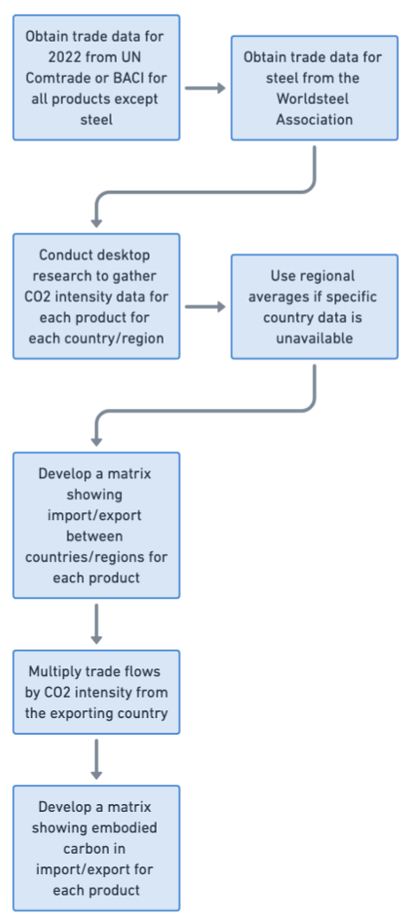
For all products except steel, the trade data for 2022 was obtained either from the UN Comtrade database (UN Comtrade 2024) or BACI trade database (BACI, 2024). For the steel trade, we used the Worldsteel Association data (worldsteel 2023).
We conducted extensive desktop research to obtain the CO2 intensity of each product for each country/region included in the product module of the tool. Numerous sources were used to gather the carbon intensity data of products. In cases where the carbon
intensity of a product for a particular country was not available, we used regional averages.
After obtaining the trade and CO2 intensity of each product, we first developed a matrix to show the import/export between different countries/regions for each product. Then, we multiplied the trade flows by the CO2 intensity of each product from the exporting country to quantify the embodied carbon in trade. This enabled us to develop a second matrix showing the embodied carbon in import/export for different countries/regions for each product. Fifigure below shows the method used in this analysis.
Below, we brielfy explain the analysis and sources of data for 4 key carbon-intensive products that are globally trded: cement, clinker, steel and aluminum.
For the cement industry, we looked into carbon embodied in the trade of both cement and clinker since both of them are traded separately in a substantial amount. Clinker is an intermediary product in the cement production process. Due to process emissions and combustion of fuel for heat, around 95% of the CO2 emitted in the cement industry is for clinker production. To reduce shipment costs, clinker is often traded instead of cement. In the destination country, the clinker is ground with some additives (e.g. gypsum, fly ash, etc.) to produce cement.s. We obtained the clinker and cement trade data from the UN Comtrade database (UN Comtrade 2024). The latest year for which the good quality trade data were available was 2019. The CO2 intensities for the cement and clinker production for different regions/countries of the world studied were obtained from the Cement Sustainability Initiative (CSI)’s Getting the Numbers Right (GNR) database, which is a voluntary, independently-managed database of CO2 and energy performance information on the global cement industry (GCCA 2022).
For the steel industry, we analyzed the carbon embodied in the trade of commodity steel. The international trade data of commodity steel were obtained from reports by the Worldsteel Association (worldsteel 2023). For the commodity steel, the latest year for which the trade data were available was 2021. The CO2 intensity of steel production in different regions/countries were obtained or estimated based on recent steel benchmarking report (Hasanbeigi 2022).
For the aluminum industry, we analyzed the carbon embodied in the trade of both primary and secondary aluminum. We obtained the aluminum trade data from the UN Comtrade database (UN Comtrade 2024). The CO2 intensity of steel production in different regions/countries were obtained or estimated based on Hasanbeigi et al. (2022) and IAI (2021).
References:
BACI, 2024, Global Trade data. http://www.cepii.fr/CEPII/en/bdd_modele/bdd_modele_item.asp?id=37
Hasanbeigi, Ali and Darwili, Aldy. (2022). Embodied Carbon in Trade: Carbon Loophole. Global Efficiency Intelligence, LLC.
Global Cement an Concrete Association (GCCA). 2022. Getting the Numbers Right (GNR). Available at
Hasanbeigi, A. 2022. Steel Climate Impact — An International Benchmarking of Energy and CO2 Intensities. Global Efficiency Intelligence. Florida, United States.
Hasanbeigi, A., Springer, C., Shi, D. 2022. Aluminum Climate Impact — An International Benchmarking of Energy and CO2 Intensities. Global Efficiency Intelligence. Florida, United States.
International Aluminium Institute (IAI). 2021.“GHG Emissions Data for the Aluminium Sector (2005-2022).”
Leontief, W. (1986). Input-Output Economics. Oxford University Press.
Miller, R. E., & Blair, P. D. (2009).Input-Output Analysis: Foundations and Extensions (2nd ed.) .Cambridge University Press
UN Comtrade. 2024. UN Comtrade Database.Available at
Worldsteel Association. 2023. World steel in figures.